Delta

Each linear RV trade is expressed as a linear combination of interest rates where the multiples denote relative value per point in local currency (so called DV01). By consensus, positive weights denote received interest rates and negative weights paid interest rates. Delta is defined as the sum of all relative DV01 weights. If delta is equal to zero, we say that the trade is DV01 neutral. If it is positive or negative, we say that the trade is net received or paid, respectively.

Notes:

• By consensus, relative DV01 weights are normalized such that at least one weight is equal to +/- 1. The DV01 volume in this interest rate serves as a unit invested in the whole trade. For example, a 2s5s flattener expressed as 1*5y - 1*2y in 50k per bp will make or lose 50k per each bp of the interest rate spread change.
• Similarly, if we decide to overweight 5y by 20% and trade 1.2*5y - 1*2y in 50k per bp, it will still make 50k per each bp change of the whole trade (trade being the number calculated as 1.2*5y - 2y). The only difference now is that a move in 5y is not translate 1:1 to the whole trade and thus a parallel curve shift will make 10k per each bp of the shift (0.2*50k).
• Some trades and analysts express butterfly with 1 in the wings and some with 1 in the middle interest rate. They are obviously two expressions for the same trade but its DV01 calibration is different.
• The fact that a trade's delta is zero does not mean that it will remain zero forever. Extreme maturities (longer than 10y) will show a second order effect called convexity and therefore originally DV01 neutral trade will become net paid or received as interest rates change.
• A classic RV trade has zero delta. This follows the conventional view that a parallel shift is the most volatile factor. However, sometimes a small residual delta may offset a trade's directional bias due to significantly different volatility in the used interest rates.
• Compared to simple interest rate spreads, butterflies have an extra degree of freedom allowing us to build a range of DV01 neutral trades using weights -1-x / 2 / -1+x. X can be set such that the trade satisfies an additional condition - minimised volatility, maximised roll/vol, or zero correlation with 10y.
• It is always strongly recommended to test a trade's sensitivity to a benchmark rate like 2y or 10y using regression chart or history chart of rolling beta and, if not intended, adjust the trade's delta to offset its directionality. DV01 neutrality does not guarantee zero market beta.

Decays to

Decays to is a level where the trade will be marked after a certain period of time (usually 3m, 6m or 1y) under the hypothetical assumption that the curve will remain unchanged. For example, 3y2y decays to 2y2y after 1y, or 18m5y decays to 5y after 18m. Using efficient market assumption, decays to can be interpreted as priced in future interest rate. It is sometimes said that the trade rolls to rather than decays to a level. For clarity, we decided to keep roll for the difference between the last level and where it decays to.

Notes:

• If the front leg is shorter than the requested decay time period, RV Goggles shows decays to as the underlying maturity, i.e. 6m5y decays to 5y in 1y time or 1i5y decays to 5y in 1y time.
• By the same token, spot starting swap decays to itself in any time, i.e. 5y decays to 5y. This is to avoid calculating carry on paid coupons which kicks in when the underlying maturity starts shortening due to passage of time. For more details relating to carry and roll see roll).
• If decays to is smaller (bigger) than last level and trade is received (paid), it will make money on a static curve because it will drift in the intended profit direction.
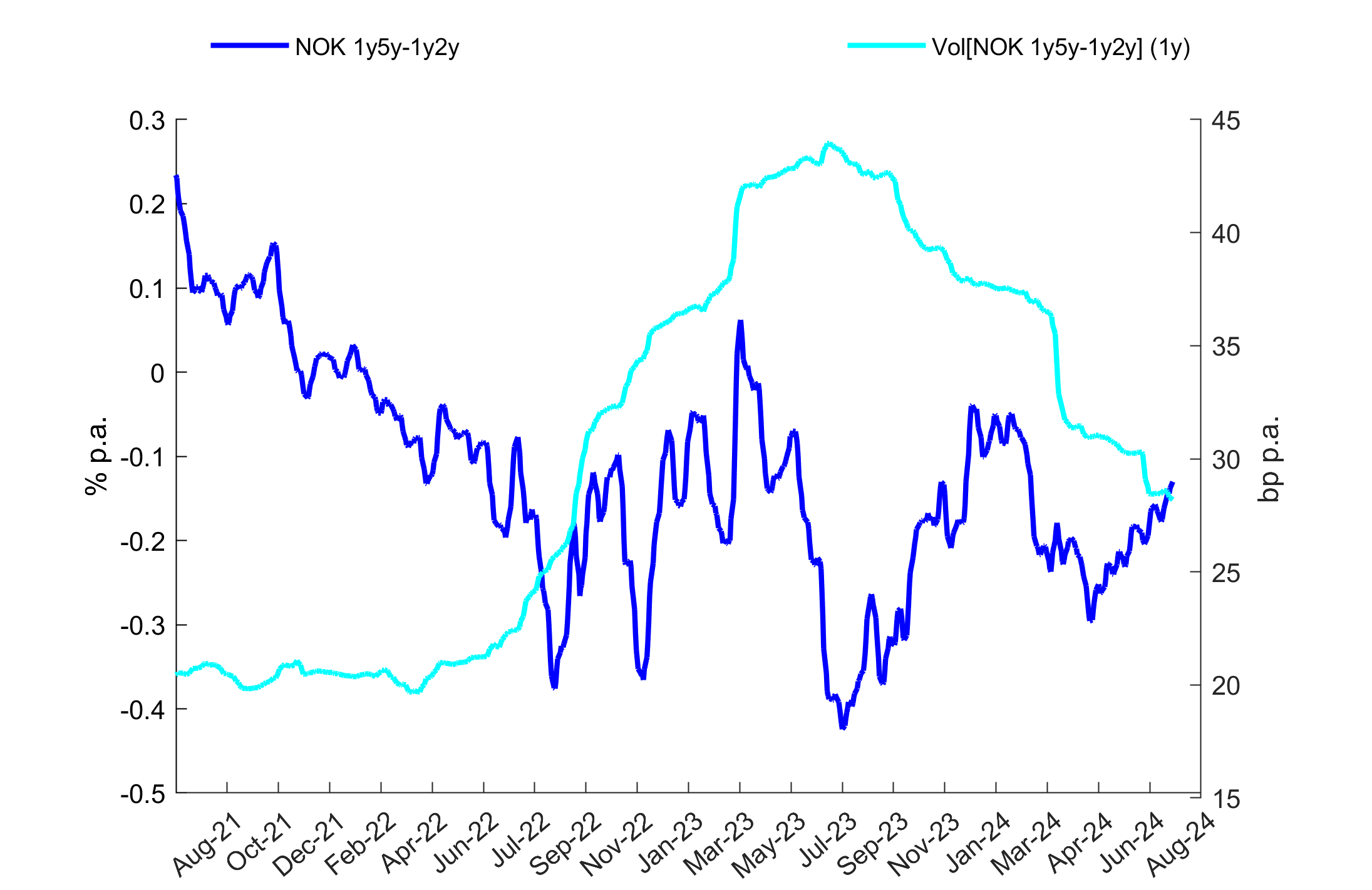
• Chart button shows by default available history of Trade 1 (as dark blue line) and 1y decays to (as light blue line).
• Chart curve shows a trade and its decays to levels along the whole available curve. Setting trade as 1y, this chart shows 1y forward curve which can be interpreted as priced in interest rate path.

Roll or Rolldown

Roll is defined as the last level less decays to level typically using 1y, 6m or 3m time period and expressed as basis points (bp) per 1y, 6m or 3m. Using this definition, roll translates into profit if the trade is received and roll is positive or if the trade is paid and roll is negative. Some traders and analysts use the term carry instead of roll but these two are not the same. While carry is physical and usually granted cash flow, roll is a hypothetical profit or loss which may disappear or even change sign, based on the curve shape at the time of the trade's unwind (profit or loss take).

Notes:

• Roll is not granted, but it is preferred to have it in the targeted direction because it can generate profit when markets are calm or liquidity is low and makes it easier to wait until the curve comes back to its usual shape.
• Similarly, if a trade has negative roll it is very likely that market positions will not be sticky and market participants will be prone to take loss on such a trade.
• Roll can be interpreted as a compensation for a position against market consensus. Some traders use roll as an indication of a crowded trade as market participants are accepting to lose on roll in exchange for a participation on an obvious (crowded) curve move. A typical example is steepener on an inverted curve.
• Roll has to be put into context with the expected holding period and the targeted curve move. Having a trade which rolls opposite to the targeted direction expresses the view that the curve will move faster and/or more than priced in to offset the negative impact of roll.
• A high roll can be a signal that the trade is equivalent or even can be replicated by a received position and vice versa.

Vol or Volatility

Volatility is a measure of the trade's dispersion. The most common way of calculating volatility is to evaluate standard deviation of daily changes in bp with a certain lookback and scaling it by sqrt(260) to express it in bp p.a. (not in bp per day). This is the definition used by RV Goggles and the definition used by most risk management systems. Under rather strong assumptions (which are often violated), volatility can be loosely interpreted as an expected drift per year. If we further assume that the underlying process is normal, we can say that with 99% probability the trade's level after one year will be within +/- 2.6*volatility from the last observed level.

Notes:

• The first strong assumption is that the underlying distribution doesn't have so-called fat tails, i.e. relatively high probability of extreme events. If this is the case, standard deviation will be a random number which will never converge no matter how long lookback we apply. The second assumption is that daily changes are independent and identically distributed, i.e. that the daily changes do not have memory and the curve dynamics does not fundamentally change over the lookback period. Despite the drawbacks volatility is widely used even if as a risk measure it often underestimates the market risk.
• Some quant analysts believe that volatility should be scaled by sqrt(360), the assumption being that the underlying market process (price formation based on flow of information) works even during weekends. Given how imprecise estimate volatility is, the difference between the two scaling factors is, at least for linear products, negligible.
• Some quant analysts are using weekly changes or weekly changes of weekly averages instead of daily changes hoping to supress the daily market noise and misquotes. While weekly moves can be cleaner, weekly data needs longer lookback and longer lookback risks a change of the underlying dynamics caused by a change of economic environment.
• Volatility as defined above is calculated on rate changes. We can apply the same approach to levels and calculate standard deviation of daily observed levels. Such calculated standard deviation is not scaled and resulting volatility is expressed in bp (not in bp p.a.). It is easier to intuitively interpret the result but there is a higher probability of violating the assumptions under which volatility gives meaningful results.
• The problem of volatility on levels or on changes may seem rather academic but becomes even more apparent if we want to measure correlation. Like volatility, correlation of two trades may be calculated on levels or changes. From RV perspective, we prefer correlation on levels (we do not mind if two trades do not correlate day-to-day) though, technically, correlation calculated on levels may not converge with increasing number of observations. RV Goggles are showing correlation on both levels and changes. If the two estimates are very different, correlation on levels should be interpreted with caution.

Range

Range like volatility is a measure of trade's dispersion over a certain lookback. It is measured as a difference between maximum and minimum and expressed in the same units as interest rates, i.e. percentage or basis points p.a. Unlike Volatility, Range is always defined no matter of the underlying distribution and there is no need for long lookbacks as it only depends on two observations. The downside is that there is no obvious scaling in time, so knowing 1 week range tells us very little about the theoretical range for 1y or longer. And further, range is sensitive to any measurement error or excessive market reaction which translates directly to reached minimum or maximum.

Notes:

• Majority of RV community is using volatility but only a minority is paying attention to details of how and why volatility is defined. Range has much smaller scope for alternative definitions. The only parameter it uses is lookback.
• Both range and Q are simplified versions of more frequently used counterparts volatility and Z. Their simplicity makes them easier to explain and replicate and they both avoid calculating second moment whose existence is sometimes questionable.

Z or Z-score

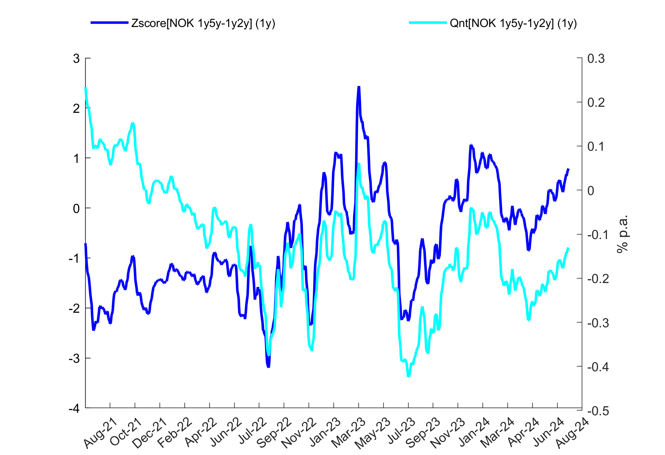
Z is the difference of the last level from its average divided by volatility.

Z ≡ (Last - Mean) / σ

The idea is to calculate a statistic which is normally distributed and thus its values can be quantified in terms of probability of occurrence. Z below -2.5 or above 2.5 is considered a signal to pay or receive, respectively, as it is associated with low probability of occurrence (units of percent of observations). Like for volatility, all these conclusions hold only under fairly strong assumptions and there are many alternative definitions. Nevertheless, Z is the most frequently used quantifier of entry and target for an RV trade.

Notes:

• It is normally assumed that lookback applied to mean and volatility is the same (which is the case for RV Goggles), but it does not have to be the case. In fact, quant analysts are often using more responsive moving average instead of a non-weighed average over the whole lookback period.
• Some analysts are adding roll to the nominator to adjust the deviation from average for expected profit or loss from time decay. The tacit assumption here is that the curve will correct to its mean and its shape (which defines roll) will be maintained which is often mutually excluding. For this reason, we prefer monitoring roll independently of the targeted level (see Roll/Vol).
• It is not entirely clear whether the denominator should be volatility on level or on changes (see notes on Vol). If we assume that the underlying trade process is mean-reverting then, in order to obtain a normally distributed statistics, we should apply volatility on levels. If it is not, then volatility on levels is meaningless. However, applying volatility on changes results in a statistics whose distribution is not obvious (in fact, we are using different processes for nominator and denominator), so Z is useless.
• The implication of the previous note is that Z should only be applied to mean-reverting trades. Thus, Z applied to a single interest rate (like 10y, for example) will most likely result in a false entry signal, as asset prices and interest rates follow non-stationary processes.
• Z is often used in connection with Principal Component Analysis (PCA). The idea is to decompose the dynamics of interest rates into non-correlated sub-processes and combining interest rates such that the combination cancels out the most volatile part. It is assumed that what remains is a mean-reverting process and thus Z is a good entry signal. Note though, that eliminating the most volatile sub-process requires at least two interest rates - one paid and one received.
• Technically, Z should follow Student's distribution with n-1 degrees of freedom, where n is the number of observations used. As n becomes large, Student's distribution converges to normal distribution, so its critical values (+/- 2.5) are automatically assessed using normal distribution.
• The usage of Z is not new. Equity technical analysts started to use so-called Bollinger Band charts in the 80s. The underlying idea, that the equity or stock index price should remain within a volatility - related band around its moving average.

Q or Quantile

Q is a scaled version of statistical quantile and is defined as the position of the last observation relative to minimum and maximum with a certain lookback (usually years). It is scaled such that Q = 1 means that the last level is at its maximum, Q = -1 at its minimum and Q = 0 at its median. Like Z, Q is a measure of entry and potential profit. Clearly, we want to receive trades with high Q and pay trades with low Q because (under the assumption of a mean reversion) we believe there is a higher probability of it reversing direction.

Notes:

• Q does not say anything about the trade's mean-reversion. The only message we can read from Q with a lookback of n-years is that the trade's last level is high or low relative to its n-years history.
• It is recommended to monitor Q with a high lookback like 5y and Q with a short lookback up to 1y. The short lookback Q indicates a recent move while the high lookback Q relates the recent move to a longer history.
• Using the definition of Q and roll, we are searching for trades with high Q and positive roll (to be received) or with low Q and negative roll (to be paid)

Roll/Vol or Roll/Rng

Roll/Vol and Roll/Rng are measures of roll per uint of risk measured by volatility and range, respectively. It can be used to compare roll of two different trades with significantly different dispersions (e.g. received/paid vs steepener/flattener). Equally, if roll has opposite direction than target, these ratios show how significant the drift is. While absolute values below 0.1 are considered negligible, values above 0.5 indicate strong roll relative to expected profit and loss generated by curve move.

Bloomberg Anywhere

The users are responsible to check if the intended Bloomberg data usage is in line with their Bloomberg Anywhere licence contract.

If you have Bloomberg Anywhere on your PC, RV Goggles can read daily Bloomberg data and synchronize it with RV Goggles interest rate data. To do that use BBG instead of curve FX, Bloomberg keyword instead of curve type, and Bloomberg ticker (or your CIX) instead of interest rate bucket. By placing 1 into the BBG row and zeros otherwise, the user can create a trade and plot the ticker alongside RV Goggles times series, analyse its correlation, or regression beta. Bloomberg tickers will show zero roll.

Further, by clicking on light-blue button Curves in the main GUI, RV Goggles will open a new window with live pricing of forward swaps. Choosing a curve using the drop-down and/or overwriting Bloomberg quote provider (like MTRT below), this application will populate the table with three spot curves: the last available RV Goggles snap (Close), last quote from the requested provider (Quote), and Estimated, which is the same as Quote but allows the user to overwrite some (or all) of the individual rates. The blue table on the right-hand side of the GUI is a small forward swap calculator. By filling in the three buckets and DV01 weights, the user can price up to three forward swaps out of the three spot curves. This is useful either for trade price refresh or for testing a trade's sensitivity to par rates.

And finally, right-click on the spot curves table offers an option Snap estimated. By clicking this option, the last curve in RV Goggles is overwritten with Estimated spot curve and the values in the main GUI are refreshed based on this curve snap. Moreover, the chosen quote provider is saved and curve refresh (using the last available quote from this provider) can now be done by a single-click on button BB Refresh in the main GUI. RV Goggles will show date and time of last refresh. The user-snap data is not saved and will be lost when the current instance of RV Goggles is closed. Reload Data from File main menu will reset the data back to RV Goggles daily snaps (i.e. Close curve).

If you do not have Bloomberg API opened on your PC, RV Goggles will automatically disable these functionalities.

Curves and their Parameters

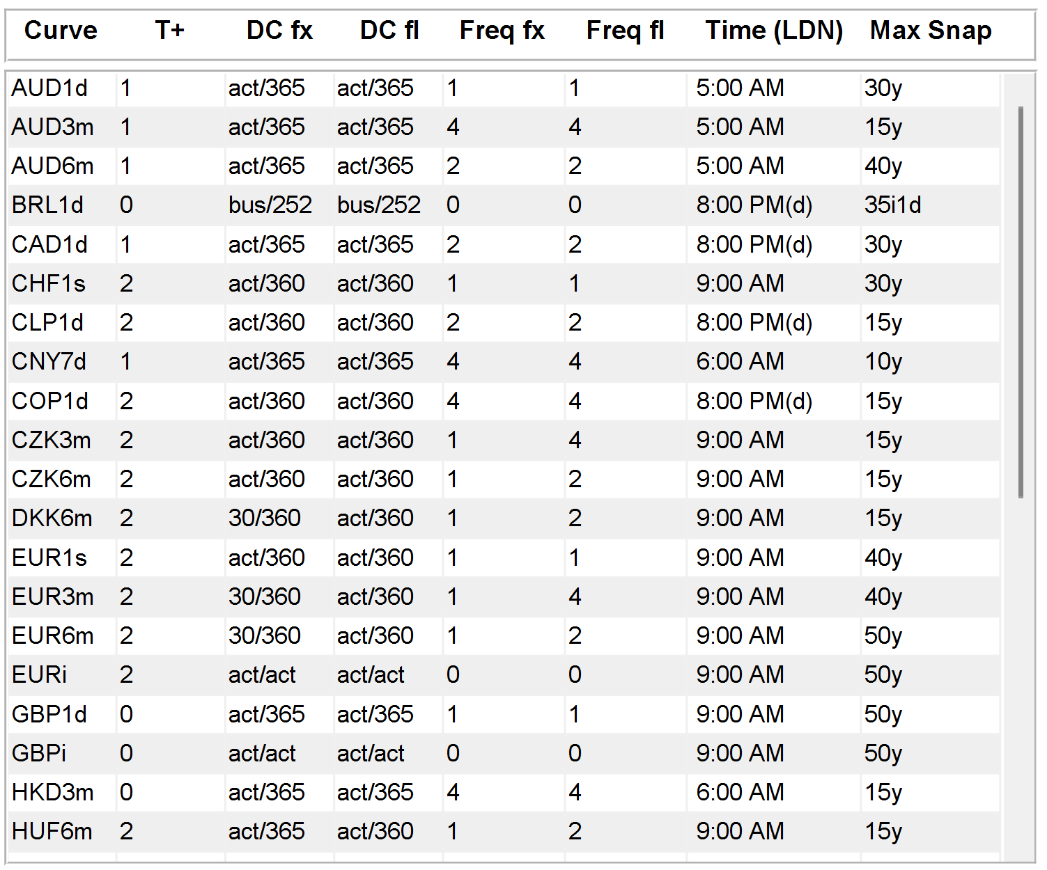
To see a list of all available curves and their parameters, click on Tools in the main RV Goggles GUI and then click on All Curves. A table of all available curves in alphabetical order will pop out. The columns show T-plus in days, day counts for fixed and floating leg, coupon frequencies for fixed and floating leg, snapping times and maximum maturity available. If the user asks for an interest rate which reaches beyond the maximum maturity, RV Goggles will return N/A. However, note that Tools also offers an item Extrapolate which is ticked off by default. If the user ticks it on, RV Goggles extrapolates the curve (log of discount curve using cubic splines) and returns a value.

Cross-Curve and Cross-Trade Comparisons

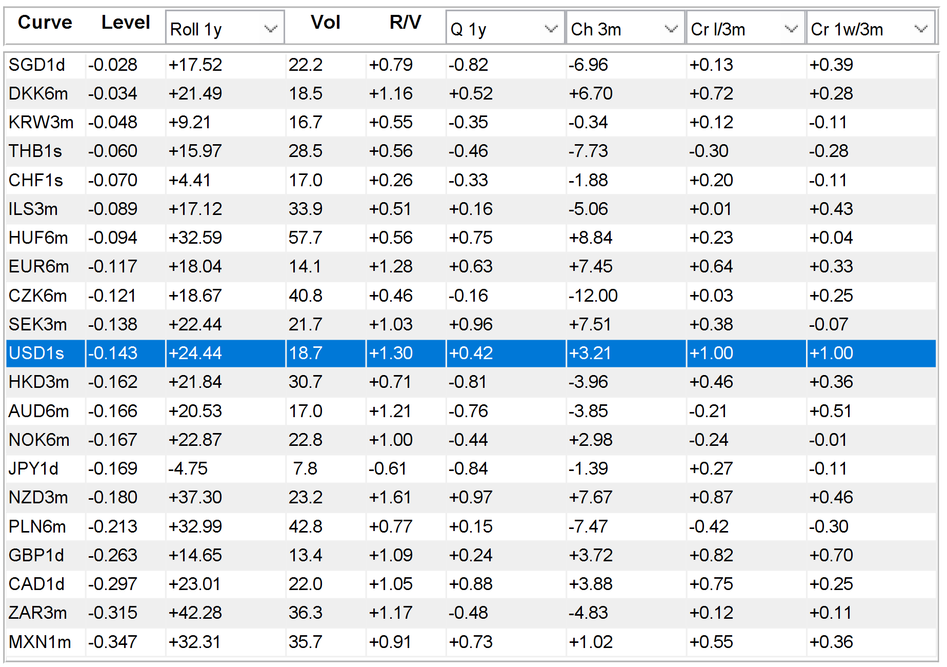
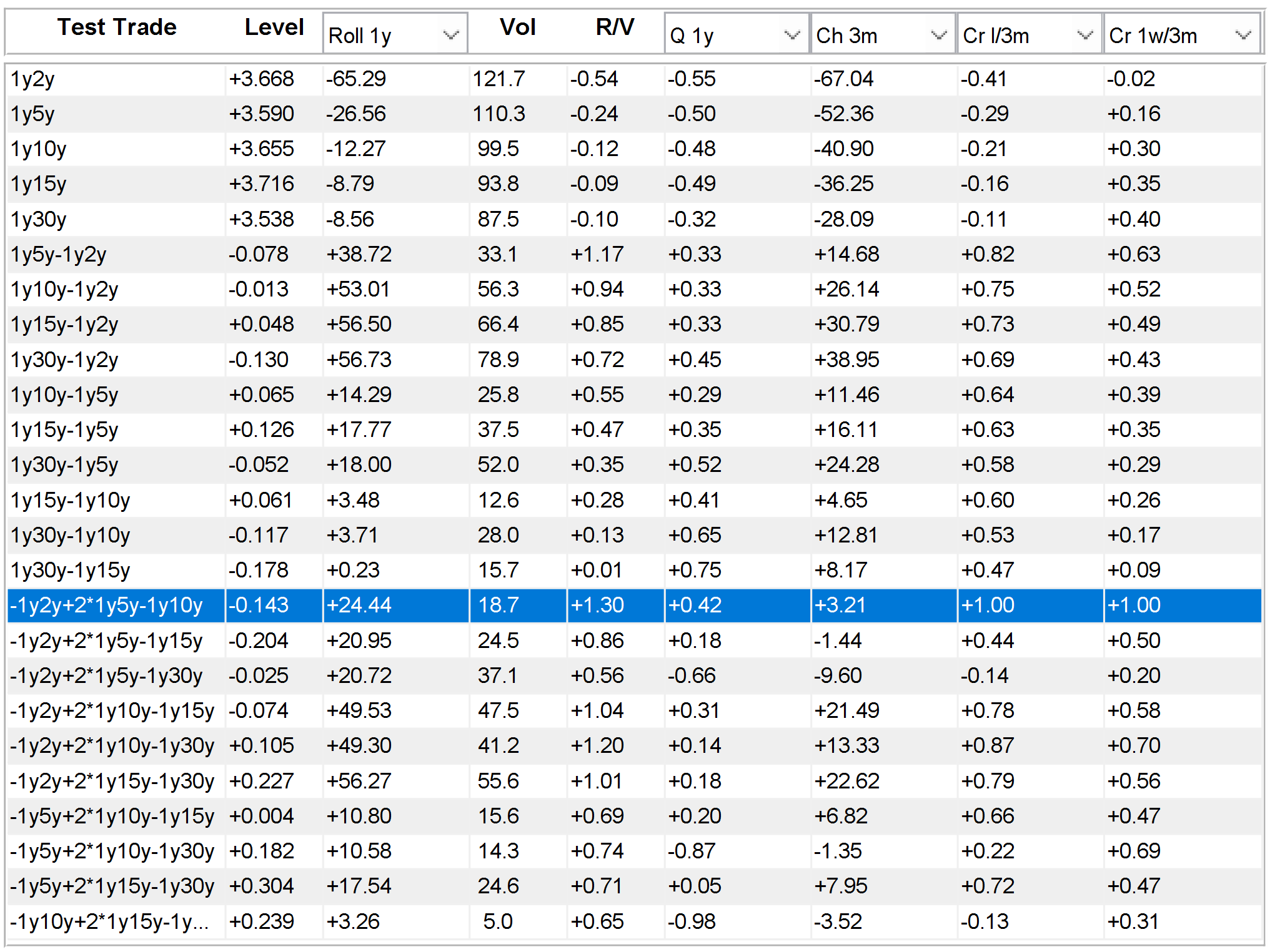
To see a comparison of one trade across all curves, right-click on the trade column in the main GUI and click on xC Table. RV Goggles will open a new figure with a table of statistics for the chosen trades and all curves which have sufficient length to price this trade. The table shows curves in alphabetical order. However, by right-clicking on the table, the user can sort the table based on any column in ascending or descending order. If the chosen trade contains more than one curve, only the first curve (top-down in the main GUI) is iterated. For example, a box AUD 1*5y - USD 1*5y will show a table of all curves' 5y spread to USD. In a similar way, the user can open xT Table comparing the chosen trade to pre-defined trades on the same curve.

Note on Principal Components Analysis

PCA is a statistical method used to decrease dimensionality of a multidimensional statistical sample. It is based on spectral decomposition of variance-covariance matrix and thus identifying the main variance drivers common to all variables of the system. Applied to a system of interest rates, the first three factors typically explain more than 90% of total variance. They are verbally described as parallel shift, slope, and curvature, and they are widely accepted as the main interest rate curve drivers (i.e. PCA factors). RV trades, like butterflies, are then built such that the first or first and second components are hedged-out so the resulting trade has strong mean-reversion and thus high probability of correction of its excessive values.

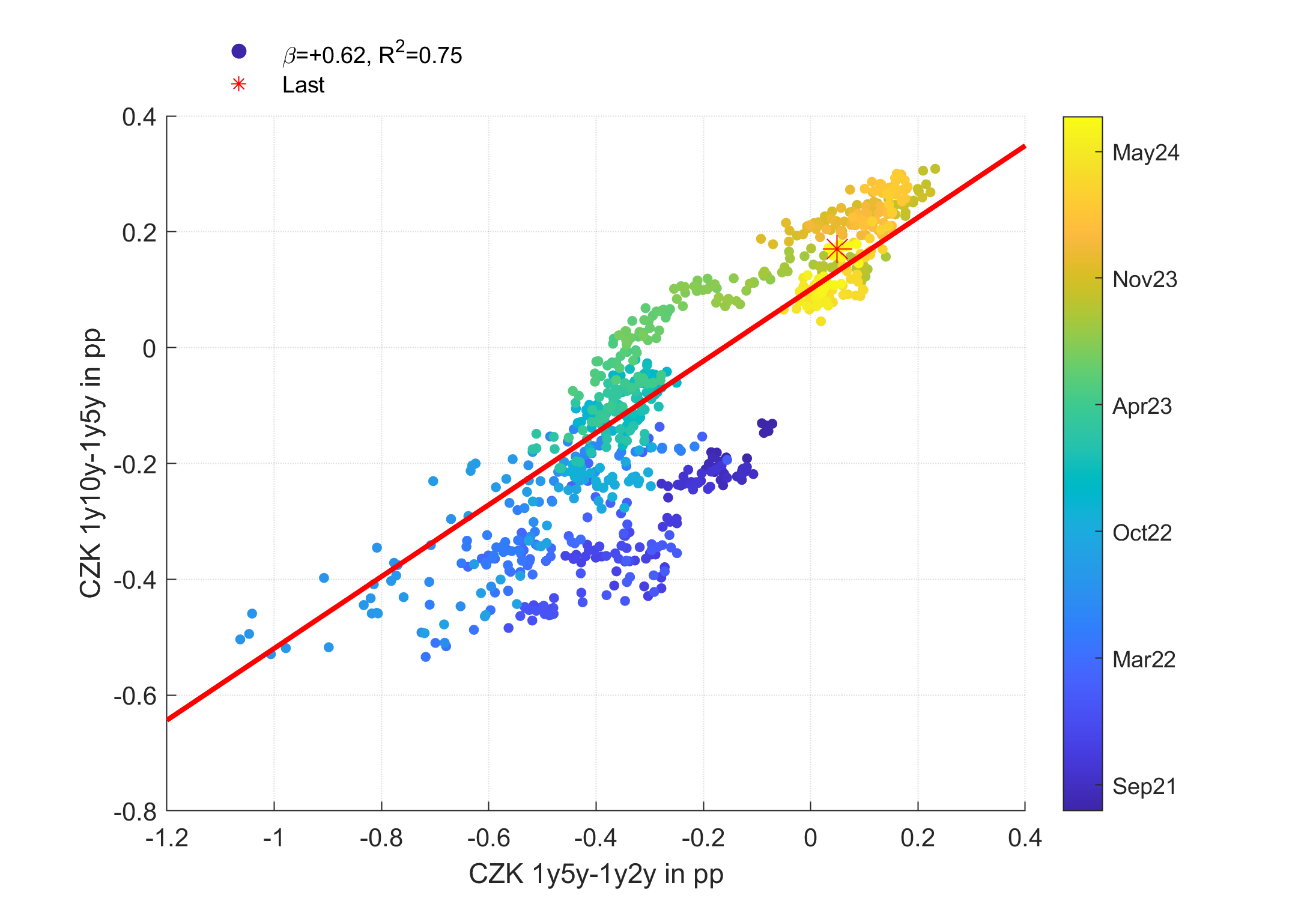
PCA is not implemented in RV Goggles but the built-in regression chart can help finding weighted butterflies which, by minimising variance of residuals, eliminate the most volatile component, pretty much like eliminating the most volatile (or trending) first principal components. Suppose that we want to build a regression-weighted CZK butterfly 2s5s10s 1y forward. Creating Trade 1 as 1y5y - 1y2y and Trade 2 as 1y10y - 1y5y, we can open regression chart and run regression

1y10y - 1y5y = α + β * (1y5y-1y2y) + ε

Choosing 1y lookback, we can find the estimated ? approximately 0.6. Plugging in 0.6 into the equation above and reshuffling all the interest rates on one side, we obtain

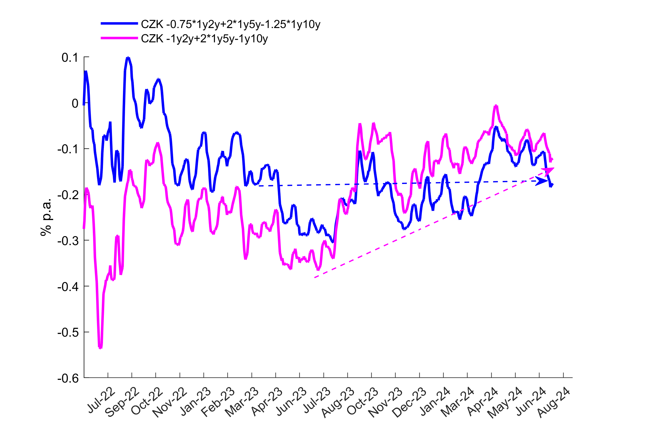
-0.6 * 1y2y + 1.6 * 1y5y - 1* 1y10y = -α - ε

To scale the relative DV01 weight in 1y5y to 2, it suffices to multiply the whole equation by a factor of 2/1.6 which translates the relative weights into -0.75 / 2 / -1.25. If fact, such butterfly is a tradable DV01 neutral expression of the regression residuum. Such butterflies have better balance of volatility of the front and back ends and thus are less volatile and cannot be replicated by front-end flattener or back-end steepener.

Even though regression does not use all available interest rates and thus does not cover the whole curve dynamics, it has one advantage over PCA. While PCA needs long lookbacks for estimation of variance-covariance matrix (typically of order 10x10), regression can work with relatively short lookbacks measured by months. Therefore, regression based DV01 weightings will be more responsive to new observations and will quickly adjust to regime changes. It is always recommended to check regression weights to understand the trade's bias when using simple pre-set weights like -1 / 1 or -1 / 2 / -1. Understanding the trade's bias (or driver) helps to predict its behaviour, to understand the reason of generating profit or loss and, if necessary, to implement the most effective hedge.

RG Goggles Installation Instructions

Once you have obtained an email with your AWS login credentials, follow the steps below to install RV Goggles on your PC.

• Create two user environment variables for your login name and login password using variables names and values sent by email. Without creating these variables, your access to RV Goggles application and its data will be rejected. Here is a hint how to create a new environment variable.
• Install Matlab Runtime version R2024a (24.1). The download is free of charge and including installation takes about 15-20min. Check that runtime has been correctly installed on your PC. Matlab Runtime default installation path is C:\Program Files\MATLAB\MATLAB Runtime.
• Create an RV Goggles target folder on your PC (e.g. "RVGoggles" in your Documents folder).
• Download gogglesV19INST.exe and move it from Downloads folder into your target folder (e.g. "RVGoggles").

   

  Download gogglesV19INST.exe

   

• Start gogglesV19INST.exe in the target folder. If you have correctly set up your environment variables and installed Matlab Runtime, it will install into the same folder two files: splash.png and gogglesV19.exe. Splash.png is Matlab logo which shows after you start gogglesV19.exe. GogglesV19.exe is RV Goggles compiled Matlab code. GogglesV19INST.exe does not install anything else and does not change your system settings.
• You may be warned by Windows that you are attempting to run an application from an unknown provider. If this is the case, click on More info and Run anyway. GogglesV19INST.exe will try to open RV Goggles after it installs the files into the target folder. If it fails (you will see en error message on screen), open the application manually by double-clicking the exe file.
• Optionally, right-click on gogglesV19.exe and create a shortcut on your desktop.
• After you start gogglesV19.exe, Matlab logo will show on the screen to confirm a launch of the application. It will disappear and after few seconds a progress bar showing the data download followed by the main RV Goggles GUI will open. The first start takes usually longer than successive starts. The data download (some 30MB) takes 6-7s. GogglesV19.exe generates a log file in the target folder where you can read potential warnings or error messages.